
2.2. Modelling specific diseases
2.2.1. Generic Disease pathway
The generic disease model is based on results from the GBD (Global Burden of Disease) 2016 project [Institute for Health Metrics and Evaluation (IHME) [82]]. The majority of diseases and injuries are modelled using DisMod-MR 2.0, a Bayesian mixed-effects meta-regression modelling tool developed for GBD analyses [Flaxman, Vos and Murray, 2015 [19]] . This tool provides estimates for incidence, remission, fatality and prevalence rate for over 300 conditions in 195 countries and territories from 1990 to 2016. Data was accessed through the web tool Epi Visualization - IHME [Institute for Health Metrics and Evaluation (IHME) [82]]
The IHME dataset provides information on incidence, fatality and remission rates for every disease. The disease pathway is modelled through three events: incidence, remission and fatality. The remission and the fatality hazard ratio are derived from the IHME database, directly. Given risk factors affect disease incidence, the baseline risk disease incidence is multiplied by a factor taking into account the risk profile of the individual (see Section 3, specifically, 4.1.2, for further details). For certain diseases – stroke, myocardial infarction, injuries – if the individual experienced a remission, he/she is at higher risk of experiencing other events (i.e. developing other diseases), such as developing a second stroke. Therefore, the model takes into account causal relationships between diseases through disease relates risk factors.
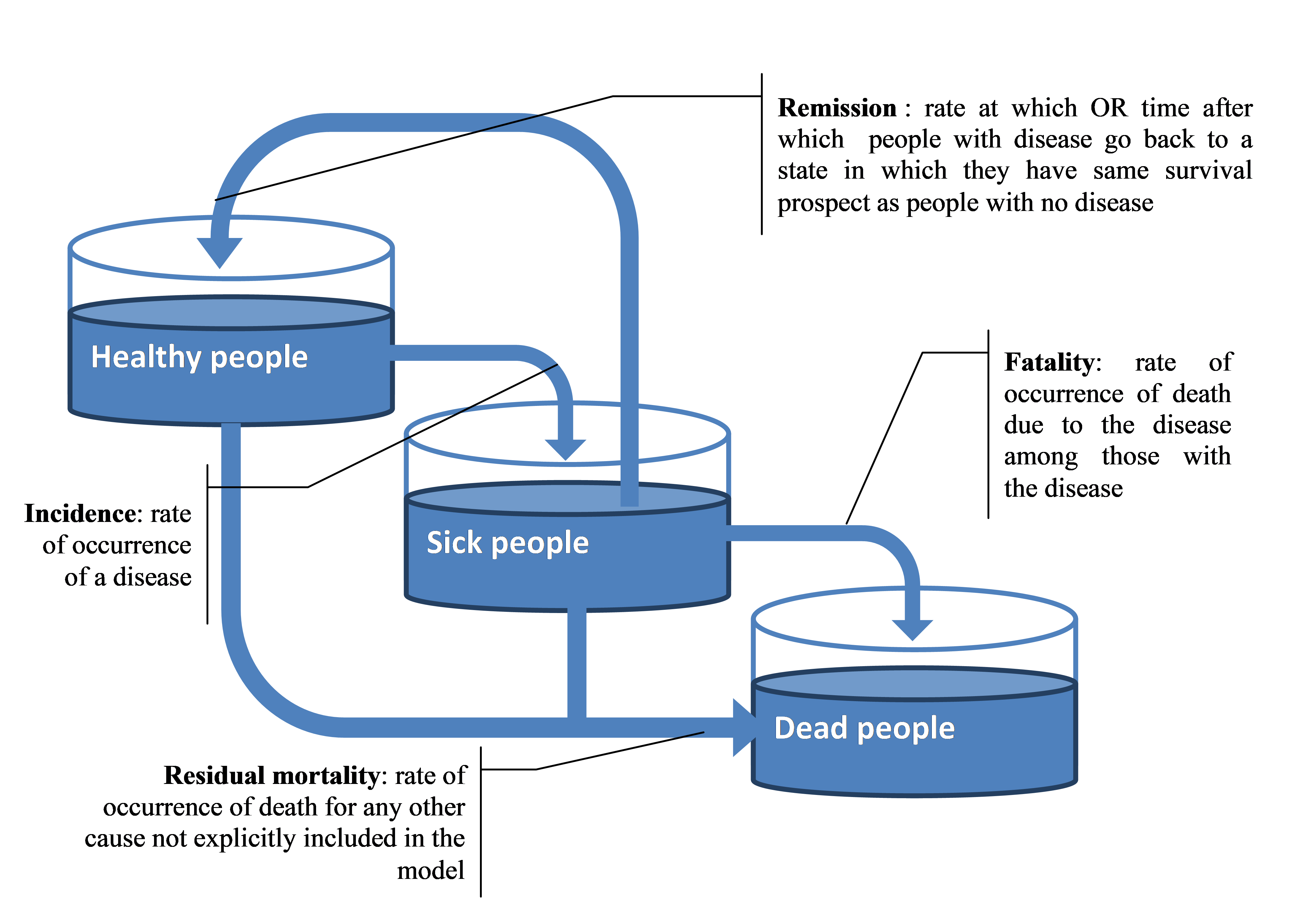
Fig. 2.1 Modelled disease pathway in the microsimulation model
For some diseases, this main model is slightly modified to take into account disease specificities.
2.2.1.1. Chronic kidney diseases
For chronic kidney disease (CKD), the disease pathway as described in Section 2.2.1 was updated to take into account stages IV and V of CKD. The IHME dataset provides access to stage IV incidence, fatality for both stage IV and V and transition rate to Stage IV to V [Institute for Health Metrics and Evaluation (IHME) [82]]. The CKD pathway, as described in Fig. 2.2, was modelled through 3 events –incidence to CKD stage IV, transition from stage IV to V and fatality whose rate depends on stage. It was assumed there is no remission for CKD.
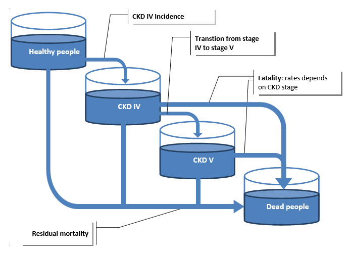
Fig. 2.2 Modelled chronic kidney disease pathway in the microsimulation model
The formula (2.1) used to compute the residual mortality is also adapted as the mortality from CKD is computed as follow:
2.2.1.2. Cirrhosis
For cirrhosis, the disease pathway as described in Section 2.2.1 was updated to take into account compensated and uncompensated cirrhosis.
The IHME dataset [Institute for Health Metrics and Evaluation (IHME) [82]] provides access to compensated cirrhosis incidence, transition rate to decompensated cirrhosis and fatality rate associated to decompensated cirrhosis (no fatality is associated with compensated cirrhosis). The cirrhosis pathway, as described in Fig. 2.3, was modelled through 3 events –incidence to compensated cirrhosis, transition from compensated to decompensated cirrhosis and fatality. It was assumed there is no remission for cirrhosis.
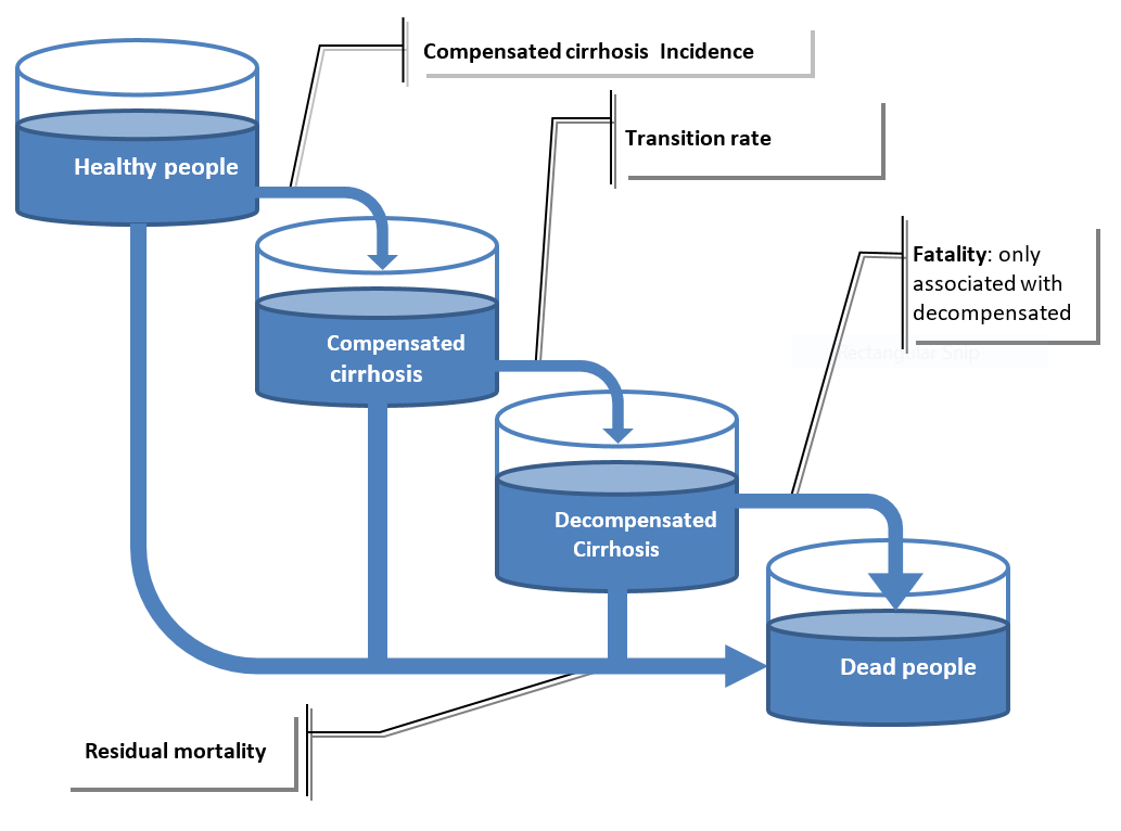
Fig. 2.3 Modelled cirrhosis disease pathway in the microsimulation model
Cirrhosis and Liver Cancer
Cirrhosis (compensated and decompensated) is a risk factor for developing liver cancer. From literature review it appears that around 50% of people developing a liver cancer had a cirrhosis. The relative risk of developing a liver cancer with a cirrhosis was estimated around 100, using the prevalence of cirrhosis (compensated and decompensated) and the incidence of liver cancer, t. Cross validity check was made using the model produced proportion of liver cancers developing with a cirrhosis.
2.2.1.3. Alcohol dependence
Alcohol dependence is model as a generic disease using the disease pathway described above in Section 2.2.1.
Adjustments were made to take into account the close relationships between dependence and alcohol use disorder (AUD). AUD is modelled as a drinking pattern (see section_alcohol_aud) and not as a disease.
It has been then assumed that individuals who do not have AUD who not be able to develop dependence.
Therefore incidence of alcohol dependence has been set to 0 in case of no AUD and divided by the prevalence of alcohol use disorder published by [Global Health Observatory (GHO) [77]] in case of AUD.
2.2.2. Cancers
To model cancers, it was assumed that cancer duration is five years: if the individual does not die within this timespan, he/she is considered fully recovered and therefore assumes the same survival prospects as those with no disease.
The cancer model pathway includes incidence, remission and death. Once the individual incurs cancer (the incidence stage), the five year survival rate for the individual is randomly determined based on the survival curve. In case of survival, the time to remission event is set at five years.
Survival probabilities are calibrated to match observed 5-year cancer mortality rates found in the literature. In case of death within the five years after the incidence stage, the time of death is modelled based on the distribution of cancer deaths.
2.2.2.1. 0-to-5 years from diagnosis
Between 0-5 years, individuals who have been diagnosed with cancer are die or survive. For those who die, the model estimates their time of death by creating a distribution of deaths. Using this distribution, the model can calculate the 5-year survival rate. Those who survived the 5-year period are considered to have entered remission and are no longer considered to have cancer.
Cancer deaths do not occur uniformly within the first five years of diagnosis - mortality is highest in the first year after diagnosis and declines exponentially.
Data from IARC was used to compute the distribution of deaths within five years post-diagnosis. This distribution was represented through the proportion of deaths which occurs every year \((w_0,w_1,w_2,w_3,w_4)\). Those weights are then used to determine the time of the death event. For example if the weights are (0.5, 0.3, 0.1, 0.07, 0.03) then 50% of deaths will occur during the first year of disease, 30% during the 2nd year and so on. The date of the death event is computed randomly.
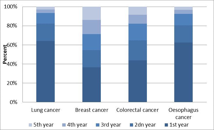
Fig. 2.4 Repartition of the deaths during the 5 years of cancers, Germany (women)
Fig. 2.4 illustrates the distribution of deaths of women within five years of being diagnosed with a certain type of cancer in Germany. For example, over 60% of individuals with lung cancer die within the first year of being diagnosed. This figure falls to below 40% for those with breast cancer. A similar type of calibration is carried out for every single country.
2.2.2.2. Five years post diagnosis
Incidence and mortality data (from IHME) are computed using survival rates at five years post-diagnosis (by gender, year and age). The deaths by cancer for a specific year and age depend on: 1) the incidence of the past five years; 2) survival rates, \(sr\), at 5 years; and 3) the distribution of deaths computed previously using IARC data.
Where
\(d\) = number of deaths
\(y\) = year
\(n\) = age
\(w\) = % of deaths for every year.
Using a piece-linear function for survival rate where age knots are fixed, the survival rate function was optimised to minimize its difference with the input mortality.
2.2.2.3. Limitations of the cancer model
There are some limitations in the model. No data was available on age-specific cancer mortality and survival. Therefore, the distribution of deaths is assumed to be constant over age. Nevertheless, the historic overall decline in cancer mortality is taken into account in the model.