
3.2.1. Alcohol
The model aims to capture two dimensions: (1) alcohol consumption, in grams or pure alcohol per day, that helps to build category of drinkers; and (2) patterns of drinking (regular, binger and alcohol use disorder). Consumption is used to classify drinkers into one of the following drinking categories:
Lifetime abstainers
Current abstainers
Moderate drinker (less than 40 grams per day for men and 20 grams for women of pure alcohol)
Heavy Drinkers (between 40 and 60 grams per day for men, and 20 and 40 grams for women of pure alcohol)
Harmful drinkers (more than 60 grams per day for men and 40 grams for women of pure alcohol).
3.2.1.1. Data inputs
The modelling of alcohol consumption relies heavily on two datasets:
The IHME dataset [Institute for Health Metrics and Evaluation (IHME) [82]]
The GISAH (Global Information System on Alcohol and Health) dataset published by in [Global Health Observatory (GHO) [78]].
From IHME, the following dimensions have been extracted by country, year and gender:
Alcohol Consumption (grams of pure alcohol per day)
Proportion of current drinkers, defined as the proportion of individuals who have consumed at least one alcoholic beverage in the last 12 months.
Proportion of binge drinkers, defined as the proportion of drinkers who have had a binge event in the past 30 days. A binge event was defined as consuming 60 grams of pure alcohol (approximately five drinks or more) in a single occasion for men and 48 grams of pure alcohol in a single occasion for women.
Proportion of former drinkers
Proportion of lifetime abstainers, defined as the proportion of individuals who have never consumed an alcoholic beverage.
From GISAH, the following dimensions have been extracted by country year and gender:
Alcohol Consumption (average daily intake in grams of pure alcohol) [Global Health Observatory (GHO) [74]]
Proportion of current drinkers [Global Health Observatory (GHO) [75]]
Proportion of binge drinkers [Global Health Observatory (GHO) [79]]
Prevalence of alcohol use disorder [Global Health Observatory (GHO) [77]]
Prevalence of dependence [Global Health Observatory (GHO) [76]]
Some unconsistencies (e.g. the prevalences of life time abstainer, current and former drinker do not sum up to 100%) and differences has be noted between the IHME and the GISAH dataset. Some can be explained like data on alcohol consumption. In the IHME dataset is self-reported whereas GISAH derives consumption from alcohol sales data. The latter is considered more accurate, however, their aggregate nature means the distribution of consumption cannot be inferred and thus cannot be used directly. However the GISAH dataset doesn’t provides estimates by age and is very limited in years. It has been then decide to rescale the IHME dataset in order to match the average estimates published in GISAH. The rescaling is based on the year where both GISAH and IHME are available. An absolute gender-specific adjustment is assumed; that is, the model reproduces the age distribution from IHME and adjusts the level of the specific measure based on GISAH data.
IHME data have also been recalibrated to ensure that Lifetime Abstainer + Current Drinker + Former Drinker = 100%. The following approach is used:
Before age 10: No Alcohol consumption. Lifetime Abstainer is set to 100%, and all the other categories to 0.
After age 18: The ‘lifetime abstainer’ proportion from IHME data is used and ‘former’ and ‘current’ proportions are calibrated to equal 100%.
Between age 10 and 18: The value of lifetime abstainer is linearly interpolated on age. The proportions of former drinker and current drinker are then calibrated to equal 100%.
3.2.1.2. Alcohol consumption
For current drinkers, alcohol consumption, i.e. the average daily intake in grams of pure alcohol, is modelled with a truncated gamma distribution following [Rehm et al., 2003 [49]]. This gamma distribution is parametrized using the average alcohol consumption \(\bar x\) by age group and gender for every country. Based on results from [Rehm et al., 2003 [49]], the relationship between \(\theta\) (the scale parameter of the Gamma distribution) and \(\bar x\) is calibrated with a power function. \(F_{AC}\) the cumulative density function for alcohol consumption is then:
with
\(\theta = \exp(0.8907 \ln(\bar x )+ 0.7001)\)
\(k =\frac{\bar x}{\theta}\)
3.2.1.3. Binge drinking, AUD and dependence
No information is found in both IHME and GISAH neither in literature to link the average daily intake of alcohol with patterns of drinking (binge, aud or dependence). A modelling approach is then used to fit the global prevalence of those different patterns while taking into account a correlation with alcohol consumption.
Binge drinking & dependence
To determine the relationship between binge drinking/dependence quantity of alcohol consumed, data from the first wave of the cross-sectional component of the Canadian NPHS (National Population Health Survey 1994-95) [Statistics Canada [88]] and several waves of the CCHS (Canadian Community Health Survey from 2000-01 to 2008-09) [Statistics Canada [87]] were used. These cross-sectional population surveys have the advantage of collecting information on drinking behaviours in the past week (seven days), which is more precise than information from the past 12 months or on a usual drinking day, as often collected in other national surveys. The CCHS and NPHS component on alcohol cover adults aged 15 and above.
In CCHS, respondents who reported drinking alcohol in the past 12 months were asked about the number of drinks in the week prior to the interview. One standard drink in Canada is assumed to contain 13.6 grams of pure alcohol. This information was used to derive the average daily intake.
The probability of being a binge drinker was derived from the question “How often in the past 12 months have you had five or more drinks on one occasion?”. Responses were dichotomized into “at least once a month” vs. “less than once a month or never”. Probabilities of being a binge drinker were then tabulated by category of quantity of alcohol consumed and by gender and age group.
In the CCHS 2003 and CCHS 2007-08, people who reported to drink five or more drinks per occasion at least once a month during the last 12 months (i.e. binge drinkers) answered the alcohol dependence questions. Alcohol dependence is defined as tolerance, withdrawal, or loss of control or social or physical problems related to alcohol use.
The CCHS questions on dependence consist of a subset of items from the Composite International Diagnostic Interview (CIDI) developed by Kessler and Mroczek (Kessler et al., 1998). And, from the answers to those questions, is derived a probability that the respondents would have been diagnosed with an alcohol dependence, if they had completed the Long-Form CIDI at the time of the interview. Probabilities of being alcohol dependent were then tabulated by category of quantity of alcohol consumed and by gender and age group.
Those probabilities were then converted into relative risks and used to model the risk of being a binge or a dependent drinker according to alcohol consumption. Those are displayed in Fig. 3.1 Fig. 3.2 (e.g. a 25-year old man who consumes 10 grams of pure alcohol per day is 3 times more likely of being a binger than if its comsumption was close to zero) - the same relative risks are applied to all countries.
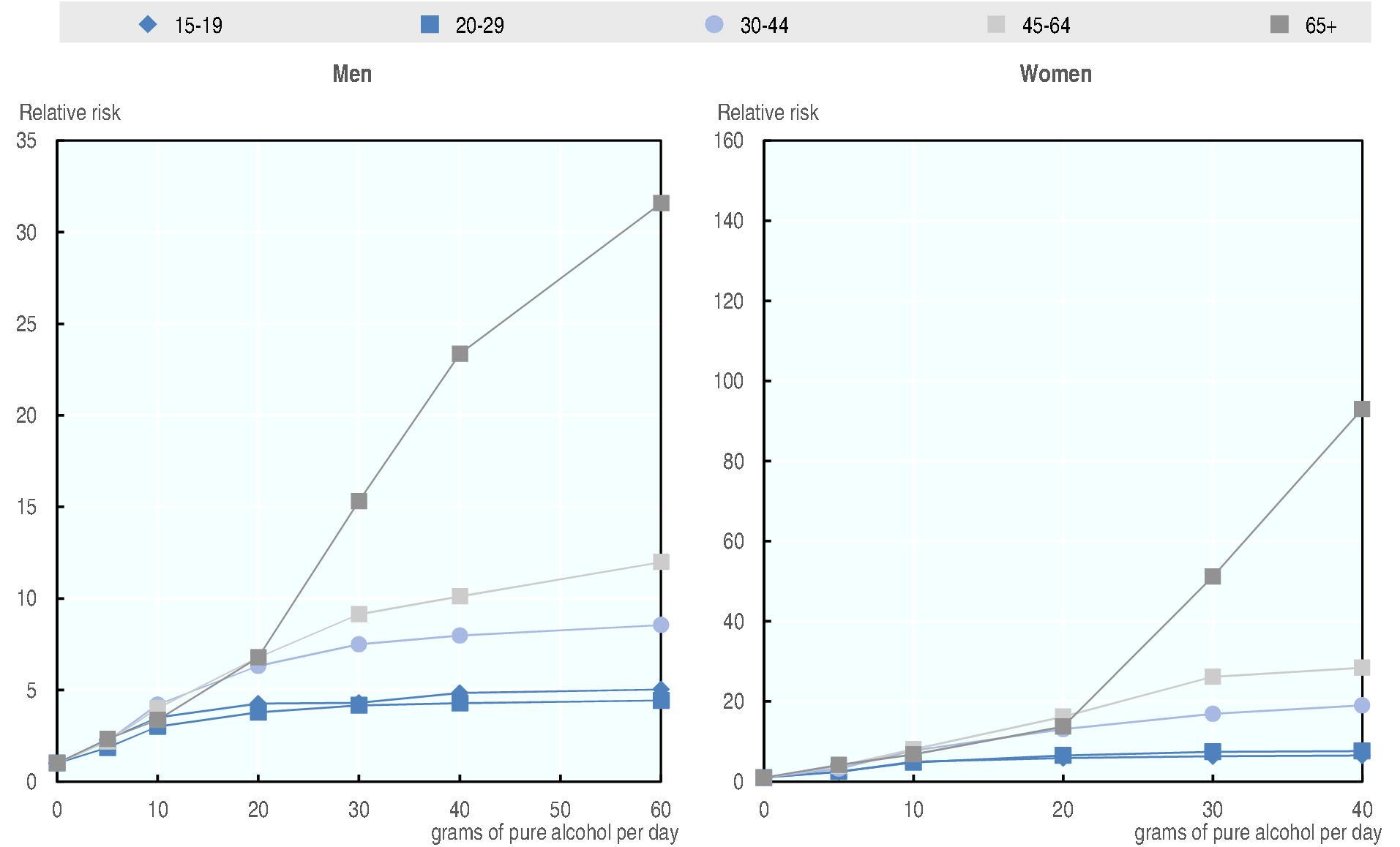
Fig. 3.1 Relative risk of being a binge drinker by quantity of alcohol consumed, gender and age group
Source: OECD 2018/19 analysis on NPHS and CCHS
Fig. 3.2 Relative risk of being a dependent drinker by quantity of alcohol consumed, gender and age group
Source: OECD 2018/19 analysis on NPHS and CCHS
Alcohol Use Disorder
Alcohol use disorder is the asymptomatic phase of dependence. It has been chosen to model it as a pattern of comsumption. As not data where available to estimate the form of the relashion ship it has been decided to use an exponential. Therefore, the probability that an individual has AUD depends on its alcohol consumption using the following equation:
\(\lambda\) has been calibrated (age and gender specific) to match the levels of AUD obtained by combining the GISAH estimates of country level, gender specific, prevalence of AUD and the IHME dataset for the age pattern. As GISAH provides estimates of AUD only for 2015, it has been assumed constant \(\lambda's\) over the years.
3.2.1.4. Simulation
At their birth, individuals are assigned as ‘life-time abstainer’ and their alcohol consumption is set to 0. This will not change until the individual experiment the drinking initiation event. After that alcohol consumption and pattern of drinking evolves as described below.
Drinking Initiation
A drinking initiation event is assigned to every individual (i.e. the year they start drinking). The event only occurs between 10 and 30 years of age (after 30, the individual remains a lifetime abstainer). The date of the event is calibrated to match the evolution of the lifetime abstainer curve.
Once the individual has passed the initiation event, his/her alcohol consumption is refreshed every year.
Alcohol consumption & Pattern of drinking
Each individual is permanently assigned into three alcohol quantiles which will determine its position in the age- and gender- specific distribution of the three dimensions of alcohol consumption. This approach means that the model is not reliant on longitudinal data to model individual drinking patterns, further, it ensures longitudinal consistency. For further information on the fixed quantile method, see [Devroye, 1986 [15]].
The first one is used to determine its position in the age- and gender-specific distribution of average daily intake of pure grams of alcohol. The second one determines his/her
Current abstention is modelled randomly based on the prevalence of current non-drinkers. If the person is a current abstainer, consumption is set to 0 for the following 12 months.
Binge Drinking
Every individual is assigned a second quantile which determines his/her likelihood of being a binge drinker. The two quantiles, one for alcohol consumption, \({q}_{1}\), and the one for binge drinking, \({q}_{2}\), are independent – the correlation between consumption and binge drinking is modelled through the joint distribution.
Alcohol Use Disorder and alcohol dependence
Alcohol use disorder is model as a pattern of comsumption. The probability that an individual has AUD depends on its alcohol consumption using the following equation:
\(\lambda\) has been calibrated (age and gender specific) to match the levels of AUD obtained by combining the GISAH estimates of country level, gender specific, prevalence of AUD and the IHME dataset for the age pattern. As GISAH provides estimates of AUD only for 2015, it has been assumed constant \(\lambda\) over the years.
3.2.1.5. Relative risks and baseline risk
The links between alcohol consumption and diseases/injuries are modelled through relative risks. Relative risks by level of consumption, age and gender were collected from IHME [GBD 2016 Risk Factors Collaborators et al., 2017 [73]] as well as the OECD Alcohol Report [Cecchini, Devaux and Sassi, 2015 [9]].
The theoretical minimum exposure measure is set to 1 for lifetime abstainer. The model also assumes that current non-drinkers have a relative risk equal to 1. For certain diseases, a moderate level of drinking may reduce the relative risk of developing a disease; the model prevents this from occurring for binge drinkers [Rehm et al., 2003 [49]]. For injuries, only binge drinkers are assumed to be at risk, therefore the relative risk is set to 1 for all non-binge drinkers.
As seen in the figure below, a moderate consumption of alcohol may have a protective effect for certain diseases. The model, however, presumes that this effect doesn’t exist for binge drinkers. The relative risk therefore, is set between 1 and the original relative risk.
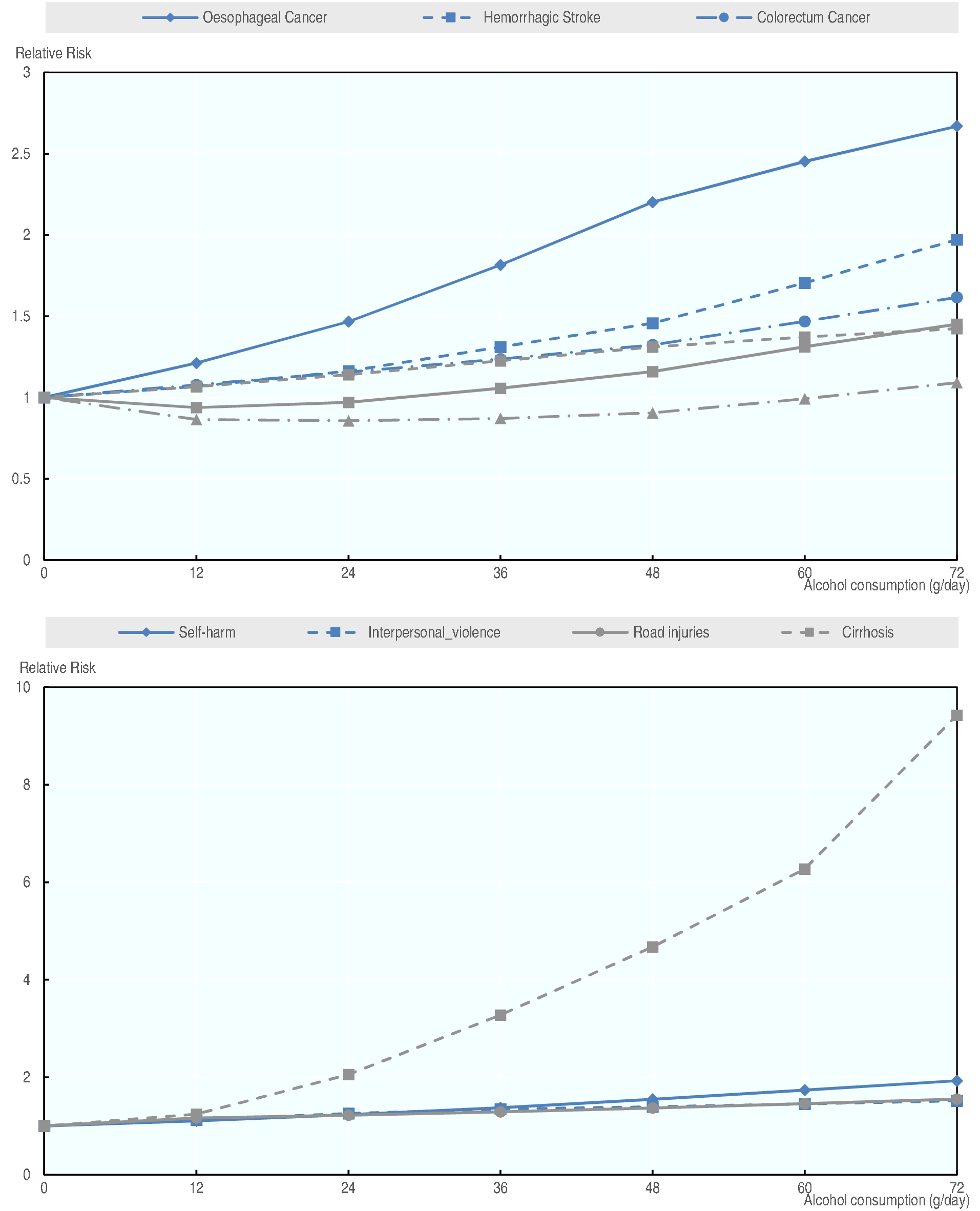
Fig. 3.3 Alcohol relative risks, for men aged 50